Demystifying the Embedding Layer in NLP

In this article, we will demystify the embedding layer in NLP, which transforms tokens - whether words, subwords, or characters - into dense vectors.

Why transform into a dense vector instead of a sparse matrix?

In NLP, one-hot encoding can be used to convert tokens into high-dimensional vectors. This method assigns a unique binary vector to each word in the vocabulary, with most of the vector’s elements being zero. While simple, one-hot encoding creates very large sparse matrices when dealing with large vocabularies, and it fails to capture semantic relationships between words. For example, ‘happy’ and ‘joyful’ would be represented as entirely different vectors, even though they have similar meanings. This lack of semantic understanding and the inefficiency of high-dimensional sparse matrices are why dense vectors, like those used in embedding layers, are preferred.

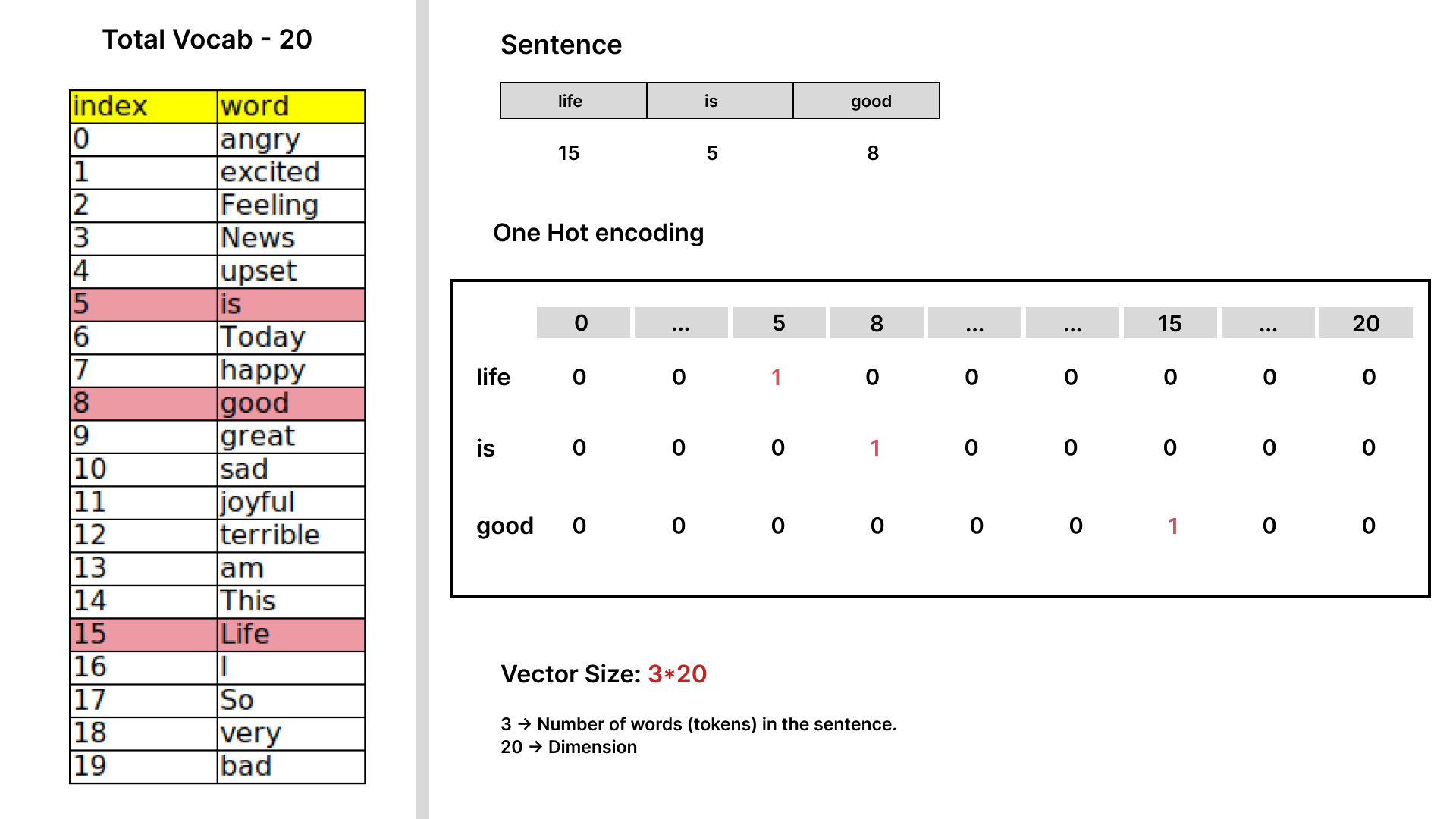Fig-1.1: Example of one hot encoding vector

• From Fig-1.1, you can see how vectors are represented using one-hot encoding. In the example provided, let’s assume a vocabulary size of 20. If we convert all the words in this vocabulary into one-hot encoding, each word will be represented as a 20-dimensional vector. However, this results in a sparse matrix—meaning most of the elements in the matrix are zeros. In a real-world scenario, with a corpus of over 500,000 unique words, one-hot encoding would create a matrix with 500,000 dimensions, where most of the elements are zero, and no semantic relationships between the words are captured.

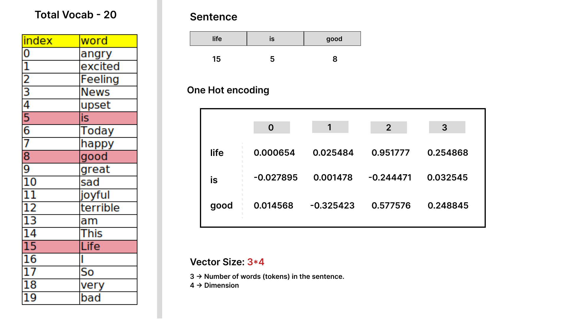_ Fig-1.2: Example of dense word embeddings.

• In contrast, Fig-1.2 shows how we can initialize embeddings with predefined dimensions, where weights are distributed across each dimension. As a learnable layer, embeddings help transform words into dense vectors that capture the semantic information of those words. This allows the model to cluster similar words together based on their distance in the embedding space. For example, words like “happy” and “joyful” would be close to each other, while “happy” and “sad” would be further apart.
• This process helps in grouping words with similar meanings. Words with the same semantic meaning, like happy and joyful, will have shorter distances between them in the embedding space, reflecting their semantic similarity.

How to train an Embedding model?

• In this section, we’ll explore how to create an embedding model that transforms words into vectors with semantic meaning. The goal of these models is to position words with similar meanings closer together in the embedding space.
• As an example, we’ll use a small dataset containing 5 positive and 5 negative sentences. We’ll treat the vocabulary from these sentences as the total set of unique words used to train our embeddings model.

positive_dataset = [
    "I am happy",
    "Feeling very joyful",
    "Life is good",
    "Today is great",
    "So very excited"
]

negative_dataset = [
    "I am sad",
    "Feeling very angry", 
    "This is bad",
    "News is terrible",
    "Feeling very upset"
]
dataset = positive_dataset+negative_dataset
target = [1]*len(positive_dataset)+[0]*len(negative_dataset)
total_vocabulary=list(set(" ".join(dataset).split(" ")))

pprint(total_vocabulary)
# output
"""
['sad', 'good', 'bad', 'Life', 'angry', 'joyful', 'This', 'So', 'News', 
'am', 'Today', 'great', 'terrible', 'excited', 'I', 'happy', 'very', 'is', 
'Feeling', 'upset']

"""

• Tokenization is the process of converting text into tokens, which are individual units of meaning. In natural language processing (NLP), these tokens can be words, subwords, or even characters, depending on the task.

  In most tokenization methods, words or subwords are converted into tokens. For example, in the word “feeling”, the word might be split into two tokens: “feel” and “ing”. This allows models to understand smaller units of language, especially when dealing with complex or compound words.

  However, for the purpose of learning, we can simplify tokenization by treating each word as a single token. This means that every word in a sentence is mapped to a unique token

• Normally, We always have the vocab size (total tokens used for training) of more than 500k tokes. For an example and learning purpose, i just used the total words in the dataset which is 19 (len(set(" ".join(dataset).split(" "))))
• We can create a dictionary where each word is assigned a unique index (token).

vocab={i:idx for idx,i in enumerate(list(set(" ".join(dataset).split(" "))))}
print(vocab)
# output
"""
{'sad': 0, 'good': 1, 'bad': 2, 'Life': 3, 'angry': 4, 'joyful': 5, 'This': 6, 'So': 7, 'News': 8, 'am': 9, 
'Today': 10, 'great': 11, 'terrible': 12, 'excited': 13, 'I': 14, 'happy': 15, 'very': 16, 'is': 17, 
'Feeling': 18, 'upset': 19}

"""

• We will iterate over each sentence in the dataset, split the sentence into words, and then replace each word with its corresponding index from the vocab dictionary.

# Encode the sentences
encoded_sentences = [[vocab[word] for word in sentence.split()] for sentence in dataset]
print(encoded_sentences)

#output
"""
[[14, 9, 15], [18, 16, 5], [3, 17, 1], [10, 17, 11], [7, 16, 13], [14, 9, 0], [18, 16, 4], [6, 17, 2], [8, 17, 12], [18, 16, 19]]
"""

• The basic training data is now ready, so let’s dive into the nn.Embedding layer in PyTorch. This layer functions as a simple lookup table, where you specify the total vocabulary size and the embedding dimension. Based on these inputs, it creates a tensor. For instance, if your vocabulary size is 20 and you set the embedding dimension to 4, a tensor of size 20x4 is generated. When you provide the index of a word, the corresponding vector from this tensor is retrieved.
• In the code snippet below, we provide an index of 1, and the model retrieves the vector for that index, which corresponds to the word “good” from the vocabulary. As you can see in the output, the embedding layer returns the correct weight vector for each token based on its index:

import torch
from torch import nn
torch.manual_seed(1)
embedding = nn.Embedding(num_embeddings=20,embedding_dim=4)
print(embedding.weight)
print("-"*55)
print(embedding.weight[1])
print("-"*55)
print(embedding.weight[[1,2,3,4]])

################################################
# Output
################################################
"""
Parameter containing:
tensor([[-1.5256, -0.7502, -0.6540, -1.6095],
        [-0.1002, -0.6092, -0.9798, -1.6091],
        [-0.7121,  0.3037, -0.7773, -0.2515],
        [-0.2223,  1.6871,  0.2284,  0.4676],
        [-0.6970, -1.1608,  0.6995,  0.1991],
        [ 0.8657,  0.2444, -0.6629,  0.8073],
        [ 1.1017, -0.1759, -2.2456, -1.4465],
        [ 0.0612, -0.6177, -0.7981, -0.1316],
        [ 1.8793, -0.0721,  0.1578, -0.7735],
        [ 0.1991,  0.0457,  0.1530, -0.4757],
        [-0.1110,  0.2927, -0.1578, -0.0288],
        [ 2.3571, -1.0373,  1.5748, -0.6298],
        [-0.9274,  0.5451,  0.0663, -0.4370],
        [ 0.7626,  0.4415,  1.1651,  2.0154],
        [ 0.1374,  0.9386, -0.1860, -0.6446],
        [ 1.5392, -0.8696, -3.3312, -0.7479],
        [-0.0255, -1.0233, -0.5962, -1.0055],
        [-0.2106, -0.0075,  1.6734,  0.0103],
        [-0.7040, -0.1853, -0.9962, -0.8313],
        [-0.4610, -0.5601,  0.3956, -0.9823]], requires_grad=True)
-------------------------------------------------------
tensor([-0.1002, -0.6092, -0.9798, -1.6091], grad_fn=<SelectBackward0>)
-------------------------------------------------------
tensor([[-0.1002, -0.6092, -0.9798, -1.6091],
        [-0.7121,  0.3037, -0.7773, -0.2515],
        [-0.2223,  1.6871,  0.2284,  0.4676],
        [-0.6970, -1.1608,  0.6995,  0.1991]], grad_fn=<IndexBackward0>)
 
"""

• We are now going to build a simple binary classification neural network, using the embedding layer as the foundation and adding two linear layers. This approach will allow us to observe how the embedding layers learn and adjust their weights as the model is trained on a larger corpus of data. After training, we can compare the initial vectors with the trained vectors in the embedding layer to see how the weights have evolved during the learning process.

torch.manual_seed(851)

# simple binary classification neural network
class TrainEmbedding(nn.Module):
    """
    A neural network module for training embeddings.

    This module uses an embedding layer followed by two fully connected layers 
    and a sigmoid activation function to produce a single output. It is designed 
    to learn embeddings from input tokens and transform them through linear 
    transformations for binary classification or regression tasks.
    """
    def __init__(self, embedding_dim, hidden_dim, vocab_size):
        super(TrainEmbedding, self).__init__()
        self.embedding = nn.Embedding(num_embeddings=vocab_size, embedding_dim=embedding_dim)
        self.linear = nn.Linear(in_features=embedding_dim*3, out_features=hidden_dim)
        self.linear_1 = nn.Linear(in_features=hidden_dim, out_features=1)
        self.sigmoid = nn.Sigmoid()

    def forward(self, x):
        x = self.embedding(x)
        x = x.flatten()
        x = torch.relu(self.linear(x))
        x = torch.relu(self.linear_1(x))
        x = self.sigmoid(x)
        return x

• In this section, we will train the model and observe how the weights of the embedding layer evolve, resulting in vectors that capture the semantic meaning of each word. This process helps group similar words based on their vector representations—words with similar meanings, like happy and joyful, will have shorter distances in the embedding space.
• Since we are using a small dataset, the model may not converge optimally, but you are encouraged to experiment with a larger corpus and a more robust architecture for better results.
• During training, we will run 100 epochs on our dataset of 10 samples, and compare the initial and final weights of the embedding layer.
• Note: The difference in weights will demonstrate how the embedding layer has learned the semantic meaning of words by adjusting the vectors. However, due to the small dataset, this approach may not yield high accuracy.

from tqdm import tqdm
import torch
import torch.nn as nn

# Ensure you're using a GPU runtime
device = torch.device("cuda" if torch.cuda.is_available() else "cpu")
print(f"Using device: {device}")

# Define the model
model = TrainEmbedding(
    embedding_dim=4,
    hidden_dim=8,
    vocab_size=len(set(" ".join(dataset).split(" ")))
)
model.to(device)  # Move model to GPU if available

# Define loss function and optimizer
loss_fn = nn.BCELoss()  # Binary Cross Entropy
temp=model.embedding.weight.clone()
print("Embedding weights before updation:\n", temp)
print("-"*50)
optimizer = torch.optim.Adam(model.parameters(), lr=0.0001)

for epoch in tqdm(range(100)):
    for idx, encoded_input in enumerate(encoded_sentences):
        model.train()        
        # Convert input and target to tensors and move them to the GPU if available
        input_tensor = torch.tensor(encoded_input).to(device)
        target_tensor = torch.tensor([target[idx]], dtype=torch.float32).to(device)

        # Forward pass
        output = model(input_tensor)

        # Compute loss
        loss = loss_fn(output, target_tensor)

        # Backward pass
        optimizer.zero_grad()
        loss.backward()
        optimizer.step()

        # Print embedding weights difference at the end of training
        if epoch == 99 and idx == 0:
            print("\nEmbedding weights difference after update:\n", (temp - model.embedding.weight))

############################################################
## output
############################################################
"""
Embedding weights before updation:
 tensor([[ 2.4533e-01,  6.2210e-01, -2.1152e-01, -1.4449e+00],
        [-1.9975e-01, -1.0331e+00,  9.8806e-01, -9.4124e-01],
        [-2.5972e-01,  9.5140e-01, -7.1059e-01, -3.0024e-01],
        [-4.6135e-01, -3.1049e-01, -7.7511e-01,  1.3188e+00],
        [ 8.3641e-01,  2.8732e-01, -1.6344e+00, -9.0064e-01],
        [-3.6750e-01, -1.5829e+00, -1.3552e+00, -7.5654e-01],
        [-3.1077e+00,  1.7162e+00,  2.9237e-01, -3.7111e-01],
        [-7.5338e-01, -6.5115e-02,  3.1420e-01,  5.4387e-01],
        [-1.2241e+00, -1.6963e-01, -1.9504e+00,  5.6253e-01],
        [ 6.6805e-01,  2.4439e-01, -1.7299e+00,  1.4293e+00],
        [-1.7114e+00, -8.5497e-01,  1.3782e+00, -6.9853e-01],
        [ 1.0628e+00,  2.0103e+00,  1.0346e+00, -2.7768e-01],
        [-1.9211e+00, -7.6792e-01, -6.8234e-01, -1.8765e-02],
        [-7.8404e-01,  1.7578e-01, -2.2046e-03,  7.0347e-01],
        [ 3.3647e-01, -6.6641e-01, -4.8028e-01,  3.3242e-01],
        [-2.0147e+00,  1.9849e-01, -1.6407e+00,  2.3918e-02],
        [ 3.1815e-01,  1.2220e+00, -3.4924e-01,  4.0813e-01],
        [-9.5412e-01,  1.5757e+00, -4.2332e-01,  5.7187e-01],
        [-1.9415e-01,  4.5028e-01,  2.3619e+00,  2.0828e-01],
        [ 2.3427e+00,  4.6440e-01, -2.7946e-01, -1.7443e+00]], device='cuda:0',
       grad_fn=<CloneBackward0>)
--------------------------------------------------
100%|██████████| 100/100 [00:01<00:00, 64.72it/s]
Embedding weights difference after update:
 tensor([[ 0.0000,  0.0000,  0.0000,  0.0000],
        [ 0.0351,  0.0380,  0.0222, -0.0246],
        [ 0.0279,  0.0266, -0.0260, -0.0257],
        [ 0.0000,  0.0000,  0.0000,  0.0000],
        [-0.0296, -0.0304,  0.0283,  0.0287],
        [ 0.0000,  0.0000,  0.0000,  0.0000],
        [ 0.0000,  0.0000,  0.0000,  0.0000],
        [ 0.0000,  0.0000,  0.0000,  0.0000],
        [ 0.0000,  0.0000,  0.0000,  0.0000],
        [ 0.0000,  0.0000,  0.0000,  0.0000],
        [ 0.0000,  0.0000,  0.0000,  0.0000],
        [ 0.0000,  0.0000,  0.0000,  0.0000],
        [ 0.0025, -0.0025,  0.0025, -0.0025],
        [ 0.0342, -0.0457,  0.0351, -0.0368],
        [ 0.0025,  0.0025, -0.0025, -0.0025],
        [ 0.0000,  0.0000,  0.0000,  0.0000],
        [ 0.0325, -0.0343,  0.0360, -0.0350],
        [ 0.0000,  0.0000,  0.0000,  0.0000],
        [ 0.0000,  0.0000,  0.0000,  0.0000],
        [ 0.0266,  0.0261,  0.0279, -0.0234]], device='cuda:0',
       grad_fn=<SubBackward0>)
"""

The output above illustrates the changes in embedding weights after training. It’s important to note that only the weights of the input index vectors are updated during training. This highlights a key characteristic of embedding layers.

Conclusion

In this demonstration, we explored a basic approach to embedding training. While this method effectively illustrates how embedding weights are updated with small datasets and simple architectures, it may not achieve high accuracy on its own. This approach serves primarily educational purposes, showcasing the fundamental mechanics of embedding layer updates.

To achieve better results, it is essential to scale this method to larger datasets and more complex architectures. Implementing advanced techniques with increased parameters can significantly improve the quality of word embeddings. Such enhancements lead to more nuanced and accurate vector representations of words, ultimately benefiting downstream natural language processing tasks and applications.

Reference:

• https://pytorch.org/docs/stable/generated/torch.nn.Embedding.html
• https://medium.com/@kumari01priyanka/embedded-layer-12cccb9a5def
• https://medium.com/@hari4om/word-embedding-d816f643140