Understanding Class Activation Maps (CAM):Part 1

This article series is divided into two parts. In the first part, I will explain the basics of Class Activation Maps (CAM) and how they are calculated. In the second part, I will delve into the working principles of Grad-CAM (Gradient-weighted Class Activation Mapping) and its implementation.

Computer Vision has undergone significant advancements in the modern era of Artificial Intelligence, evolving from simple handcrafted feature extractors to deep models that can extract relevant features, resulting in significantly improved performance. Unlike earlier models that were transparent in their working mechanisms, state-of-the-art deep models achieve high accuracy at the cost of interpretability. The field of explainable AI (XAI) has emerged to address this trade-off between performance and interpretability. XAI aims to unravel the decision-making process of complex black box models in a human-interpretable manner. By providing explanations, XAI techniques can enhance user trust and enable the adoption of opaque models in safety-critical domains such as healthcare and finance, where transparency is essential.

In practice, DL models are often viewed as black boxes that take in a dataset and give a task-specific output: predictions in image classification, captions in image captioning, and more. For example, in image classification, you optimize the model for prediction accuracy. Adding a layer of interpretability in a convnet model will be helpful for many use cases. For example, if we build a model to predict a certain medical condition from x-rays, we can use explainability to check whether the relevant part of the x-ray is used for predicting the medical condition.

To explain the ConvNet model, Zeus et al. introduced the Class Activation Map (CAM), which identifies the discriminative regions of a class in an image. Instead of using a fully connected layer, CAM utilizes the feature map to find these regions. This method can be applied to existing models, but it requires the model to contain a Global Average Pooling (GAP) layer before converting it to a fully connected layer. To overcome this limitation, Ramprasaath R. Selvaraju introduced Grad-CAM, which can be applied to any model without changing the architecture, providing a highly class-discriminative saliency map.

To understand Grad-CAM, it’s essential to grasp how CAM works. CAM is useful for identifying which regions of an image contribute to a classification decision. Papers like GoogleNet introduced Global Average Pooling (GAP) to address overfitting, using it instead of flattening the entire final feature map in a model backbone.

Implementation of Class Activation Map (CAM):

Step-1: To begin, select a trained model and provide an input image containing the target class you wish to analyze. For instance, in Figure 1.1, we pass an image of a cat to the classifier. The model’s output, Y6, correctly predicts the image as a cat.

Figure 1.1

Step-2: Essentially, Y6 for the “cat” class is the result of summing the weighted activations of neurons connected to that specific class. In the second step, our focus is on isolating the weights exclusively linked to the class or features that contribute to the classification of cats, as illustrated in Figure 1.2.

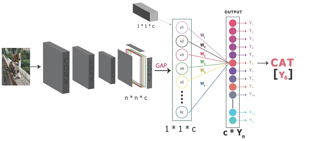Figure 1.2

Step-3: To calculate the Class Activation Maps (CAM) for a specific class, such as the “Cat Class” (Y6​), we utilize the weights associated with that particular class along with the final feature map derived from backbone architectures like Inception or ResNet

In Figure 1.3, we zoomed out to illustrate the layers involved in calculating the Class Activation Maps.

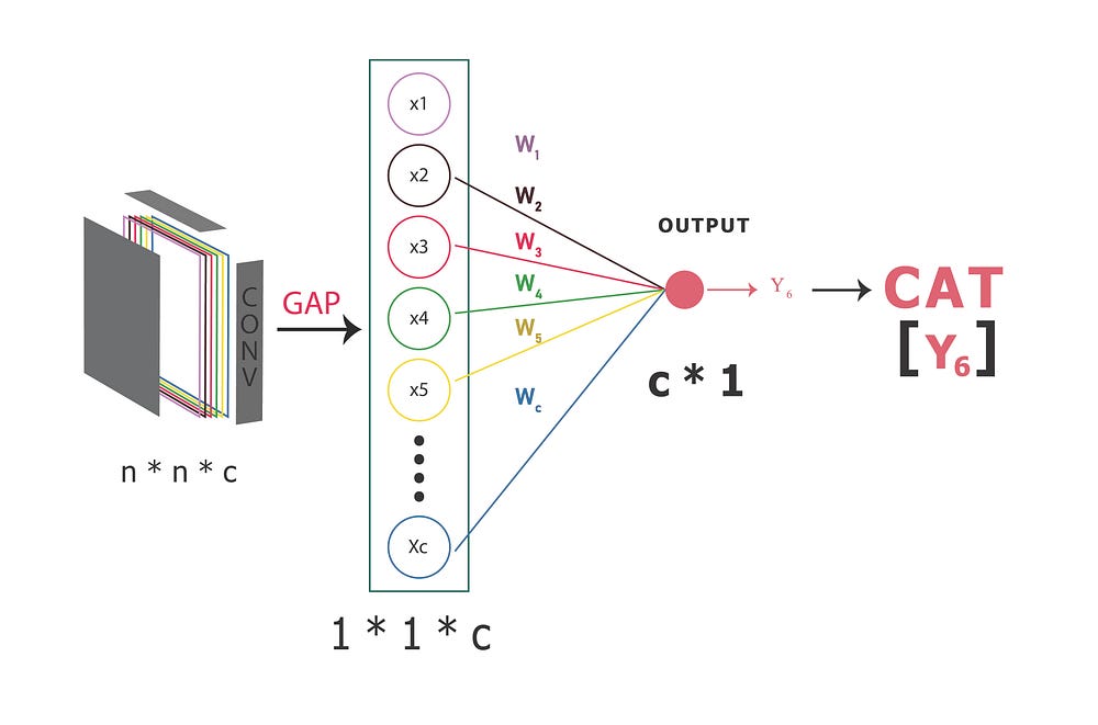Figure 1.3

Step-4: After applying Global Average Pooling to the final feature map, we obtain 1x1 vectors with the same dimensions as the final convolution layer feature map (n×n×c). To compute the CAM, we perform a weighted sum of the final convolution layer. This necessitates splitting out the specific feature map along with its corresponding weights separately, as depicted in Figure 1.4.

Figure 1.4

Step-5: The Class Activation Map (CAM) is generated by taking a weighted sum of each feature map, where the weights correspond to the importance of each feature map for a particular class. These weights are multiplied with their respective feature maps and then summed up to create the CAM. This CAM highlights discriminative regions in the input image, which can be resized and overlaid onto the original image for visual interpretation during testing, as shown in Figure 1.5.

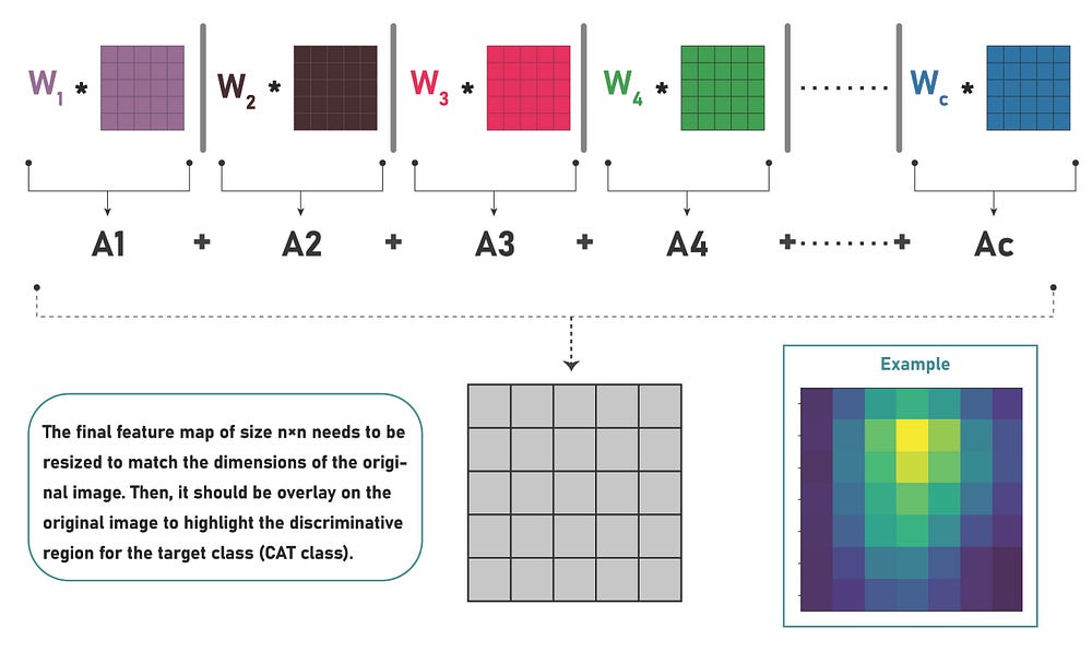Figure 1.5

CAM Implementation Using PyTorch.

Step 1: Initialise and load a pre-trained ResNet-18 model and move it to the GPU for faster processing.

import torchvision.models as models  

# Load the pre-trained ResNet-18 model and move it to the GPU
model = models.resnet18(pretrained=True).cuda()  

model = model.eval() 

Step 2: Initialise and preprocess the image by resizing, center cropping, converting it to a tensor, and normalizing it.

# Import necessary modules for image transformations and handling
import torchvision.transforms as transforms
from PIL import Image

# Define normalization transform with mean and standard deviation values
normalize = transforms.Normalize(mean=[0.485, 0.456, 0.406], std=[0.229, 0.224, 0.225])

# Define a transformation pipeline for preprocessing: resize and center crop
PIL_tops = transforms.Compose([transforms.Resize(256), transforms.CenterCrop(224)])

# Define a transformation pipeline for converting image to tensor and normalizing
tensor_tops = transforms.Compose([transforms.ToTensor(), normalize])

# Open an image file
img = Image.open("/content/input.jpg")

# Apply the resizing and center cropping transformations
cropped_img = PIL_tops(img)

# Apply the tensor conversion and normalization transformations
trans_img = tensor_tops(cropped_img)

# Add a batch dimension and move the image tensor to the GPU
model_img = trans_img.unsqueeze(0).to("cuda")

print(model_img.shape) # torch.Size([1, 3, 224, 224])

Step 3: Need to initialise the hook the get the feature map of the last layer as shown in the figure 1.4 .

# Initialize an empty dictionary to store intermediate outputs
conv_data = {}

# Define a hook function to capture the output of the final feature map of the ResNet backbone
def __hook(module, inp, out):
    conv_data["output"] = out

# Register the hook to the final feature map layer of the ResNet backbone (layer4)
model.layer4.register_forward_hook(__hook)

Step 4: To identify the discriminating regions in an image, you’ll first need to provide an image containing a cat. Once you pass this cat image through the model, you can access the final feature maps through hooks and retrieve the weights from the saved model. With these, you can compute the weighted sum of the final convolutional layer to generate a class activation map highlighting important regions in the image that contribute to the prediction of the ‘cat’ class.

# Get the output shape of the model after passing the transformed image through it
output_shape = model(trans_img.unsqueeze(0).to("cuda")).shape

# Extract the output of the convolutional layer
conv_layer_output = conv_data["output"]
conv_layer_output = conv_layer_output.squeeze(0)

# Retrieve the weights of the fully connected layer corresponding to the 'cat' class
fc_weights = model.fc.weight
cat_class_idx = 282  # Index of the 'cat' class in the ResNet-18 model
cat_fc_weights = fc_weights[cat_class_idx].unsqueeze(1).unsqueeze(1)

# Compute the weighted sum of the final convolutional layer
final_conv_layer_output = cat_fc_weights * conv_layer_output
class_activation_map = final_conv_layer_output.sum(0)

Step 5: To visualize the Class Activation Map, you’ll need to resize the CAM from its original size of 7*7to match the size of the input image, which is typically 224 * 224. Once resized, you can overlay the CAM onto the original image to highlight the important regions identified by the model.

import numpy as np
import torch.nn.functional as F
import matplotlib.pyplot as plt

# Resize the CAM array to match the size of the original image tensor
cam_resized = F.interpolate(class_activation_map.unsqueeze(0).unsqueeze(0), size=tuple(model_img.shape[-2:]), mode='bilinear', align_corners=False)

# Convert the CAM tensor to a NumPy array
cam_np = cam_resized.squeeze().cpu().detach().numpy()
cam_expanded = np.expand_dims(cam_np, axis=2)

# Convert the original image tensor to a NumPy array
img_np = np.array(img.resize((224,224)))

# Display the overlaid image
plt.imshow(img_np)
plt.imshow(cam_expanded, alpha=0.5, cmap='jet')
plt.show()

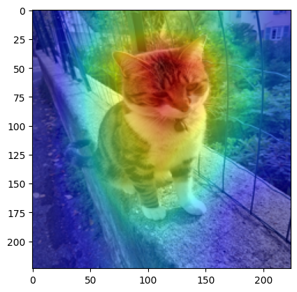Output from the step-5

I’ve included a GitHub link (https://github.com/sri-dhurkesh/Class-Activation-Maps.git) for the implementation using PyTorch. In the next part we can delve into the working principles of Grad-CAM (Gradient-weighted Class Activation Mapping) and its implementation.