Relative Position Bias

Relative position bias, introduced in the Swin Transformer research paper, enhances the Absolute Positional Encoding mechanism by effectively capturing positional information within image patches. Positional encoding is essential for conveying the spatial relationships of patches in image-based tasks, enabling the model to understand the relative arrangement of different parts of an image.

In the Swin Transformer, the concept and implementation of relative position bias can initially appear challenging and are not elaborately explained in the paper. This article aims to bridge that gap, offering a clear understanding of relative position bias and its implementation. By the end of this article, readers will have a solid grasp of how relative position bias functions and how it is implemented in the Swin Transformer repository.

Relative Position Bias with 3x3 Patches

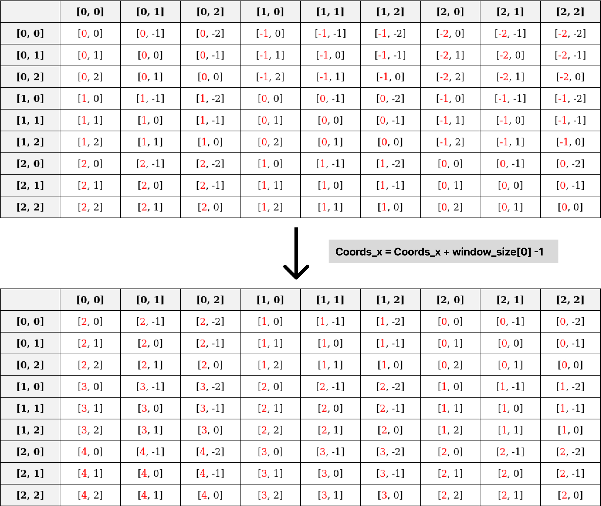
Consider having 3x3 patches of input (window_size=M=[3,3]), represented in the following image. Each cell corresponds to its respective indices, e.g., [0,0], [0,1], …, [2,2].

Relative Position Index Table

There are a total of 9 patches where each patch relates to all others. The relative position index table illustrates these relationships. For instance, the first index [0,0] has relationships with all patches. Each cell in the table represents the distance along each axis, calculated as [x1-x2, y1-y2]. These values lie within the ranges [-M[0]+1, M[0]-1] and [-M[1]+1, M[1]-1] along the x-axis and y-axis, respectively. For our example, this range is [-2,2] for both axes.

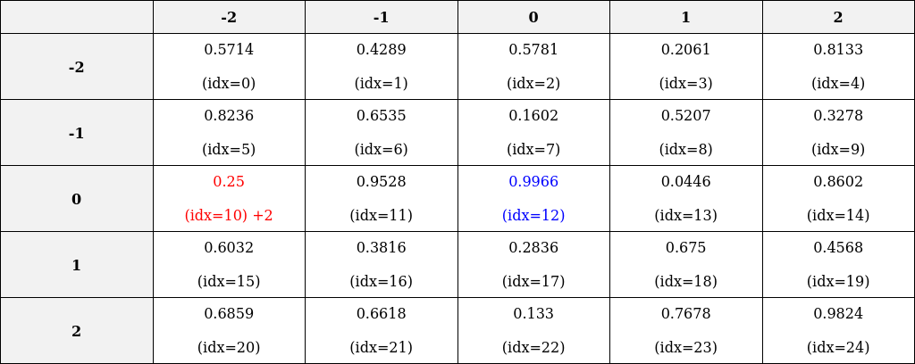
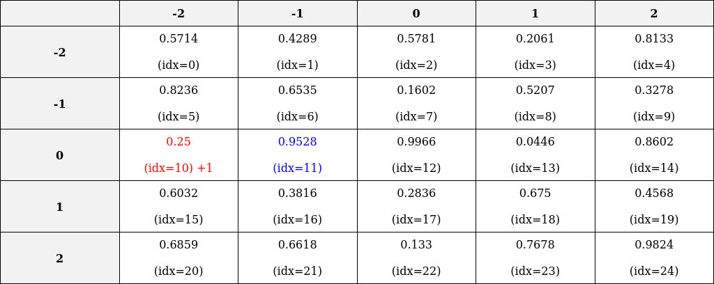
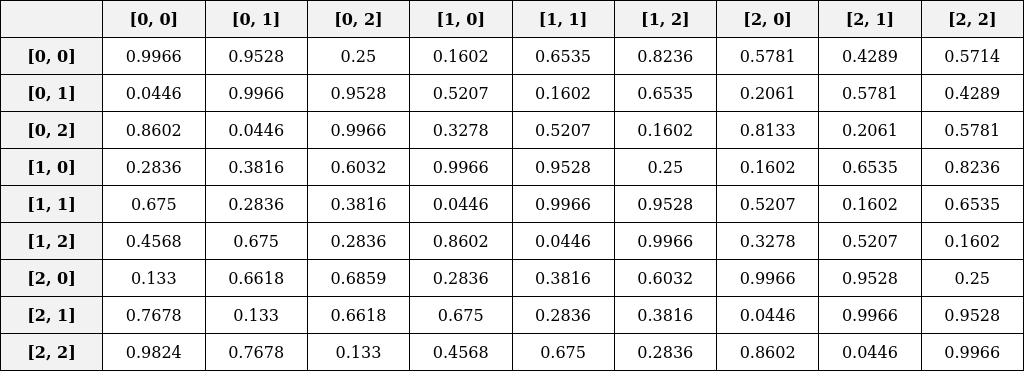
Learnable Relative Position Bias Table

We create a learnable relative position bias table where the distances range from -2 to 2 along each axis. Below is an image of this table. Index values denote positions in the flattened 1D array, while float values represent the learnable weight values. This corresponds to the following code from the Swin Transformer repository.

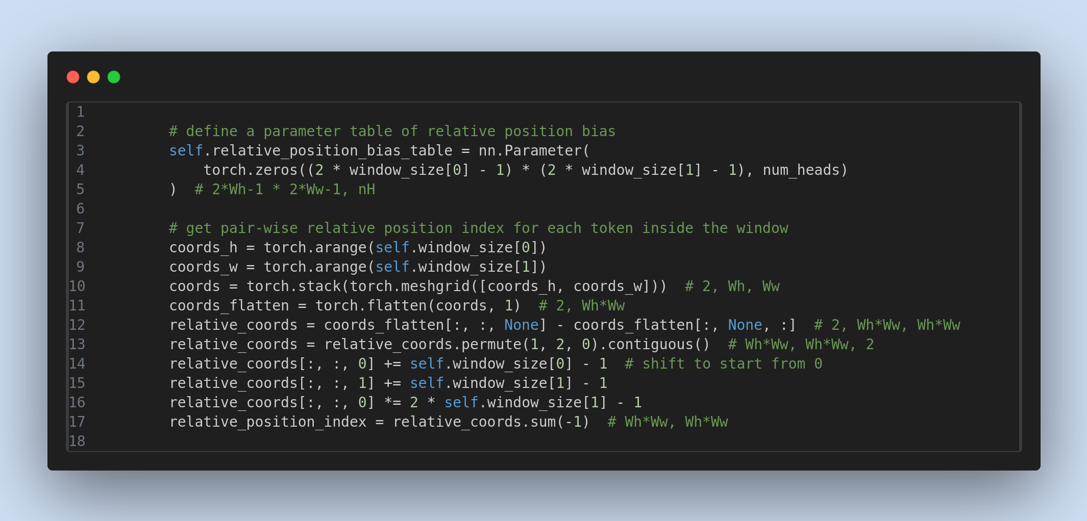
# define a parameter table of relative position bias
 self.relative_position_bias_table = nn.Parameter(torch.zeros((2 * window_size[0] - 1) * (2 * window_size[1] - 1), num_heads))  # nH=1

Filling the Bias Table

The relative position index table is populated with values from the bias table. For instance, the [0,0] entry in the relative position index table corresponds to the [0,0] entry in the relative position bias table, which is located at index idx=17 in the flattened array. To calculate the correct flattened index, we adjust the values in the relative position index table to start from 0.

Shifting Values for Index Calculation

1. Shift Along the x-axis: Add window_size[0]-1 to each value along the x-axis:

   relative_coords[:, :, 0] += self.window_size[0] - 1  # Shift to start from 0
   

   

2. Shift Along the y-axis: Similarly, add window_size[1]-1 to values along the y-axis:

   relative_coords[:, :, 1] += self.window_size[1] - 1  # Shift to start from 0
   

   

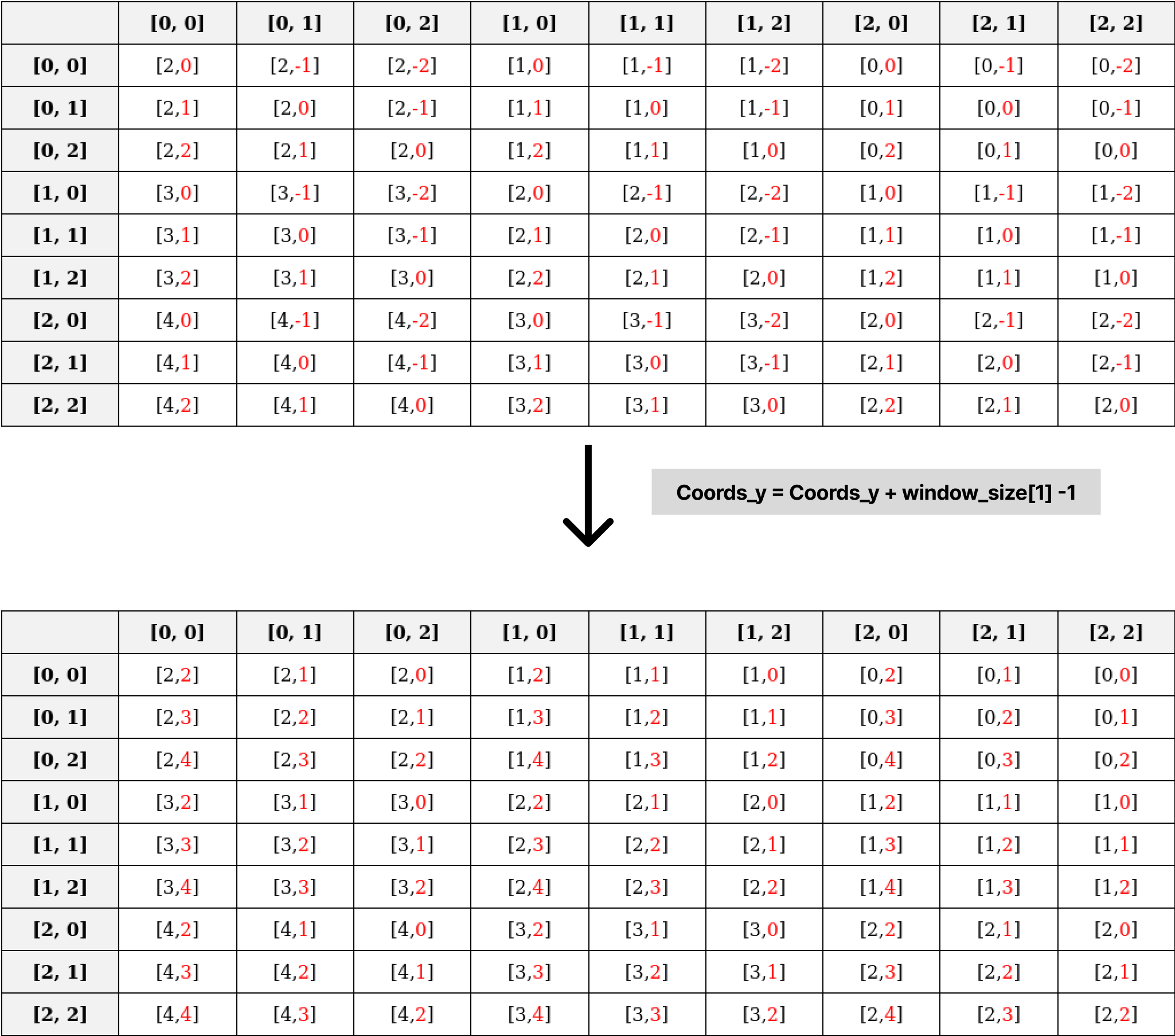
After applying these transformations, the updated relative position index table is:

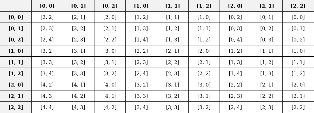
Calculating Flattened Indices

The x-axis values indicate how far to move in the flattened table. For example, [2,2] in the index table corresponds to 10 (calculated as 2 * (2 * 3 - 1) = 10).

relative_coords[:, :, 0] *= 2 * self.window_size[1] - 1

The final index is derived by adding x-axis and y-axis values:

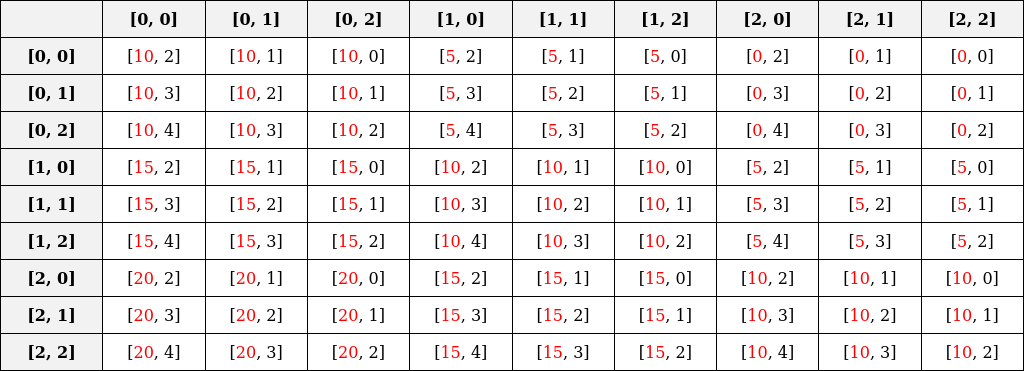
• From the above table, the x-axis element at the index [(0,0), (0,0)] is 10, which represents how much index need to move in flattened index. The y-axis element, 2, denotes the offset from this 10th index.
  • Reference image: we take the value of the [0,0]th row and [0,0]th column, which is [10,2]. Here, 10 indicates how much to move in the flattened index to get the first element in a row, and 2 adds the offset to the first element index.

  

  • Reference image: we take the value of the [0,0]th row and [0,1]th column, which is [10,1]. As a result, we get the 11th index.

  

• By adding both axes, we can get the index of the relative position bias:

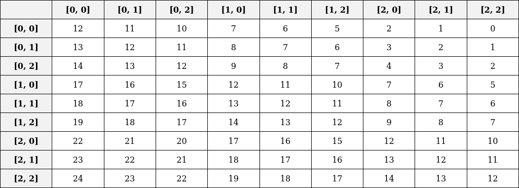
Finally, we retrieve the specific index data from the relative position bias table:

In conclusion, relative position bias effectively captures positional information within image patches, enhancing the Swin Transformer model’s performance. The learnable relative position bias table captures relative distances between patches, and the model learns to weight these distances during training. This mechanism complements the absolute positional encoding, providing a more comprehensive understanding of spatial relationships in images.

Note

The Python code snippets referenced above are directly adapted from the official Swin Transformer repository.

References

• Swin Transformer research paper: https://arxiv.org/abs/2103.14030
• Swin Transformer repository: https://github.com/microsoft/Swin-Transformer/blob/main/models/swin_transformer.py
• https://www.youtube.com/watch?v=Ws2RAh_VDyU